Here \(g\) is the loop gain of the fixed-point form \(x = F[p(x)]\), not the rate gain \(\partial(dx/dt)/\partial x\) used for stability.
The series needs \(|g| < 1\), but as the equilibrium shift for a sustained change, \(\frac{\text{Direct Effect}}{1-g}\) holds whenever \(g < 1\).
Fixed Points (Equilibria)
System dynamics are often understood relative to their equilibria (or fixed points).
If \(X_{t+1} = F(X_t)\), equilibria occur where \(F(X_t) = X_t\).
If \(\frac{dx}{dt} = f(x)\), equilibria occur where \(f(x) = 0\).
In other words, a system at an equilibrium will stay at an equilibrium.
Stability of Systems
Single-Equation System
If our model consists of one differential equation, \[\frac{dX}{dt} = F(X)\]
then the equilibria are the solutions to \(F(\hat{X}) = 0\).
Stability to Small Perturbations
Now suppose we perturb the system slightly from an equilibrium \(\hat{X}\) to \(\hat{X} + \Delta X\).
Let \(X(t)\) be the solution with this new initial condition and define \[X(t) = \hat{X} + \Delta X(t).\]
How can we analyze the behavior of the system after this perturbation?
Taylor Approximation
For a small perturbation, we can linearize the system around the equilibrium \(\hat{X}\) using the Taylor approximation \[F(\hat{X} + \Delta X) \approx F(\hat{X}) + \Delta X \left.\frac{\partial F(X)}{\partial X}\right|_{\hat{X}}.\]
Simplifying Taylor Approximation
But then since \(\hat{X}\) is time-independent and \(F(\hat{X}) = 0\):
\[
\frac{d[\Delta X(t)]}{dt} \approx \Delta X \left.\frac{dF(X)}{dX}\right|_{\hat{X}}
\]
Implications for Stability
If \(\frac{dF}{dX} < 0\), then \(\Delta X\) will decay to zero, \(X\) will return to \(\hat{X}\), and the system is stable.
If \(\frac{dF}{dX} > 0\), then \(\Delta X\) will grow, \(X\) will diverge from \(\hat{X}\), and the system is unstable.
General Model Form
Suppose our model consists of a system of differential equations
Construct a matrix \(\mathbf{A}\) (the Jacobian) with elements \[a_{ij} = \left.\frac{\partial F_i(X_1, X_2, \ldots, X_n)}{\partial X_j}\right|_{(\hat{X}_1, \hat{X}_2, \ldots, \hat{X}_n)}\]
and a vector \(\mathbf{\Delta X} = [\Delta X_1, \Delta X_2, \ldots, \Delta X_n]^\top\).
The eigenvalues of \(\mathbf{A}\) determine the stability of the system:
If all eigenvalues have negative real parts, the system is stable.
If any eigenvalue has a positive real part, the system is unstable.
If any eigenvalue has a zero real part and non-zero imaginary part, the system is degenerate and solutions oscillate around the equilibrium (sometimes called marginally stable).
Stability for Single-Equation System
If we only have one equation, this is simpler:
Stability and Resilience
Can think of stable equilibria as suggesting “resilience”: small disruptions to the system state will fade away with time and the system will stabilize.
Unstable equilibria: small shocks amplify and the system will deviate from its “typical” state.
Generalization to Difference Equations
Suppose instead of a system of ODEs, we have a system of difference equations:
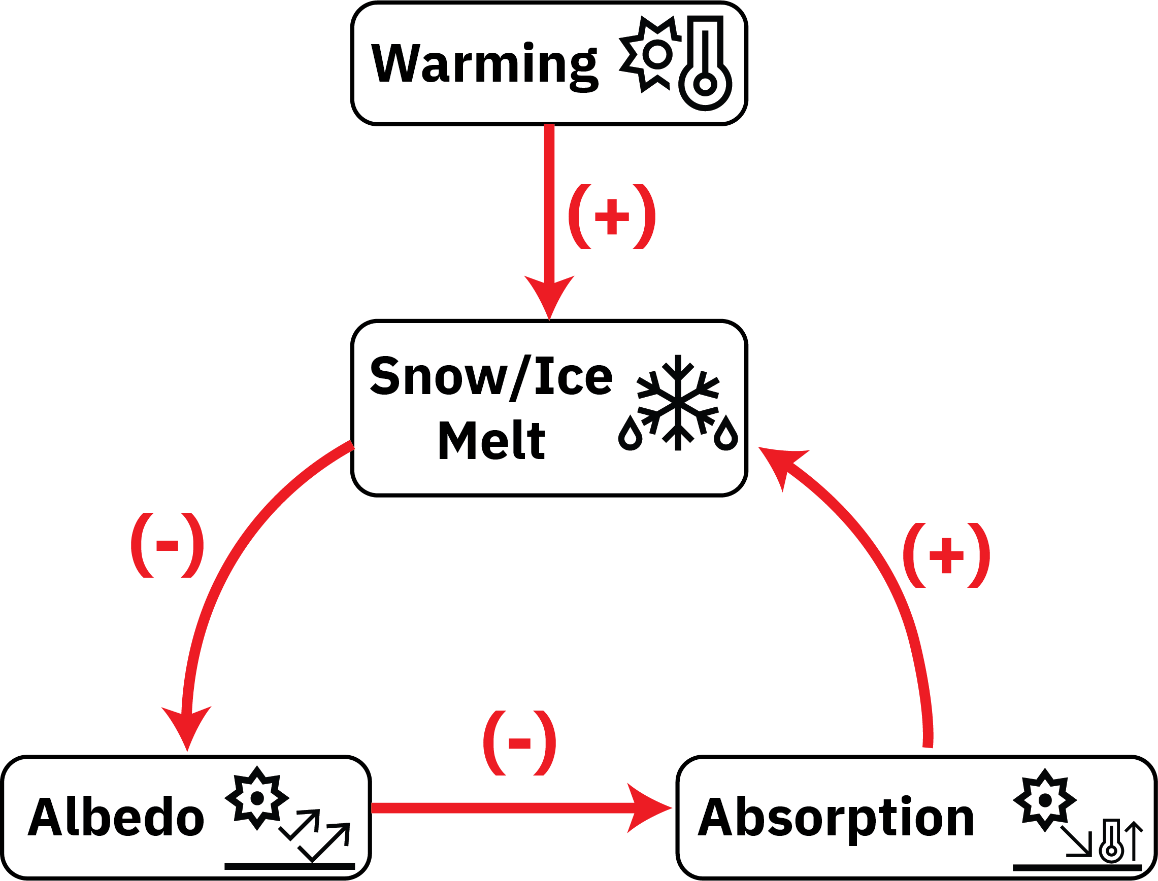
So the total feedback is \(g_{total} = g_{IA} + g_{out} \approx 0.04\).
Total Climate Model Feedback
To Sum:
When \(\alpha\) is constant (\(T < -10^\circ\text{C}\) or \(T > 10^\circ\text{C}\)), the total feedback is negative (\(g_{out} \approx -0.03\ \text{yr}^{-1}\)): a perturbation shrinks about 2.5% a year.
When \(\alpha\) can vary (\(-10^\circ\text{C} < T < 10^\circ\text{C}\)), the total feedback is positive (\(g_{total} \approx 0.04\ \text{yr}^{-1}\)): a perturbation grows about 4% a year, so an equilibrium here (\(T = 7.55^\circ\text{C}\)) is unstable.